# setup fonts
showtext_auto()
showtext_opts(dpi = 300)
font_add_google("Oswald", "oswald")
# setup colors
alpha_col <- 0.5
palette_name <- "Alkalay1"
# get country basemap
world <- rnaturalearth::ne_countries(scale = "medium", returnclass = "sf")
# basemap
bsm <-
ggplot(data = world) +
geom_sf(data = world, fill = "gray95", colour = "gray80") +
geom_sf(
data = dat_sf,
aes(size = capacity, color = titles_won),
alpha = alpha_col
) +
geom_text_repel(
data = dat_sf,
aes(label = team, geometry = geometry),
stat = "sf_coordinates",
force = 5,
family = "oswald",
) +
# Europe bounding box
coord_sf(
xlim = c(-15, 60),
ylim = c(20, 65),
expand = FALSE
) +
scale_size(
range = c(4, 12),
name = "Arena capacity",
breaks = c(5000, 10000, 15000),
labels = comma,
guide = guide_legend(
title.position = "top",
title.hjust = 0.5,
override.aes = list(alpha = 1, color = "gray30")
)
) +
scale_color_moma_c(
palette_name = palette_name,
name = "Total titles Won",
guide = guide_colorbar(
barwidth = unit(5, "cm"),
barheight = unit(0.5, "cm"),
title.position = "top",
title.hjust = 0.5,
alpha = alpha_col + 0.2
)
) +
theme_void(base_family = "oswald") +
theme(
legend.position = c(0.82, 0.80),
legend.direction = "horizontal",
legend.box.just = "center",
legend.title = element_text(size = 14),
text = element_text(size = 12)
)
#bsm
# scatter inset
scatter_inset <- ggplot(
dat_sf,
aes(x = capacity, y = titles_won, colour = titles_won)
) +
geom_point(alpha = alpha_col + 2, size = 3) +
geom_text_repel(
data = dat_sf |> filter(titles_won > 0),
aes(label = team),
size = 4,
family = "oswald"
) +
scale_colour_moma_c(
palette_name = palette_name
) +
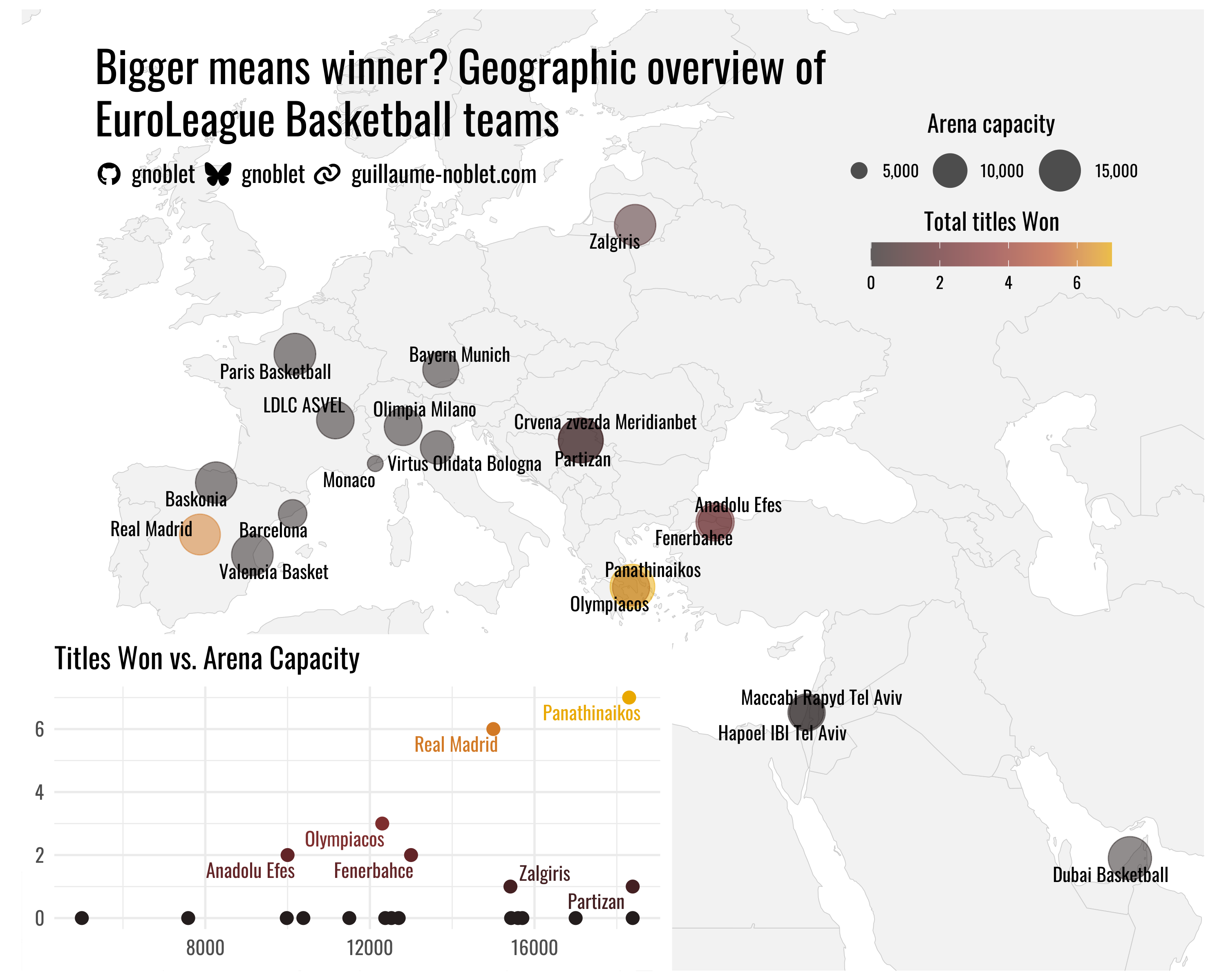
labs(title = "Titles Won vs. Arena Capacity", x = NULL, y = NULL) +
theme_minimal(
base_size = 14,
base_family = "oswald"
) +
theme(
legend.position = "none"
)
# titles
title <- "Bigger means winner? Geographic overview of EuroLeague Basketball teams"
subtitle <- branding(
github = "gnoblet",
bluesky = "gnoblet",
website = "guillaume-noblet.com",
text_size = "14pt",
icon_size = "14pt",
text_family = "oswald",
text_color = "black",
icon_color = "black"
)
caption <- "Data: EuroLeague Basketball | TidyTuesday October 7"
combined_plot <- bsm +
inset_element(
scatter_inset,
left = 0,
bottom = 0,
right = 0.55,
top = 0.35
) +
inset_element(
ggplot() +
geom_textbox(
aes(
label = title
),
family = "oswald",
x = 0.02,
y = 0.95,
hjust = 0,
fill = NA,
box.color = NA,
box.padding = unit(c(0, 0, 0, 0), "pt"),
width = unit(0.65, "npc"),
size = 9
) +
geom_textbox(
aes(
label = subtitle
),
family = "oswald",
x = 0.02,
y = 0.86,
hjust = 0,
fill = NA,
box.color = NA,
box.padding = unit(c(0, 0, 0, 0), "pt"),
width = unit(0.6, "npc"),
size = 5
) +
theme_void(),
left = 0,
right = 1,
bottom = 0,
top = 1,
align_to = 'full'
)
# save
ggsave(
"week_40.png",
plot = combined_plot,
width = 10,
height = 8,
dpi = 300
)