# Fonts
font_add_google("Roboto Condensed", "Roboto Condensed")
showtext_auto()
showtext_opts(dpi = 300)
# Create breaks for x-axis (every two weeks approximately)
spring_breaks <- c(46, 61, 75, 92)
spring_labels <- c(
"Mar 15",
"Apr 1",
"Apr 15",
"May 1"
)
# Spring migration tile plot with dark theme and ggplot2 4.0 features
p_spring <- ggplot() +
# horizontal line every 5 years
geom_segment(
data = data.frame(
y = seq(1995, 2024, by = 5),
xmin = 31,
xmax = 95
),
aes(x = xmin, xend = xmax, y = y),
color = "white",
linewidth = 0.4
) +
geom_text(
data = data.frame(
y = seq(1995, 2024, by = 5),
x = 96,
label = seq(1995, 2024, by = 5)
),
aes(x = x, y = y, label = label),
color = "white",
size = 4.5,
hjust = 0
) +
geom_tile(
data = dat_spring,
aes(x = spring_day, y = year, fill = observations),
linewidth = 0.1,
colour = "white",
) +
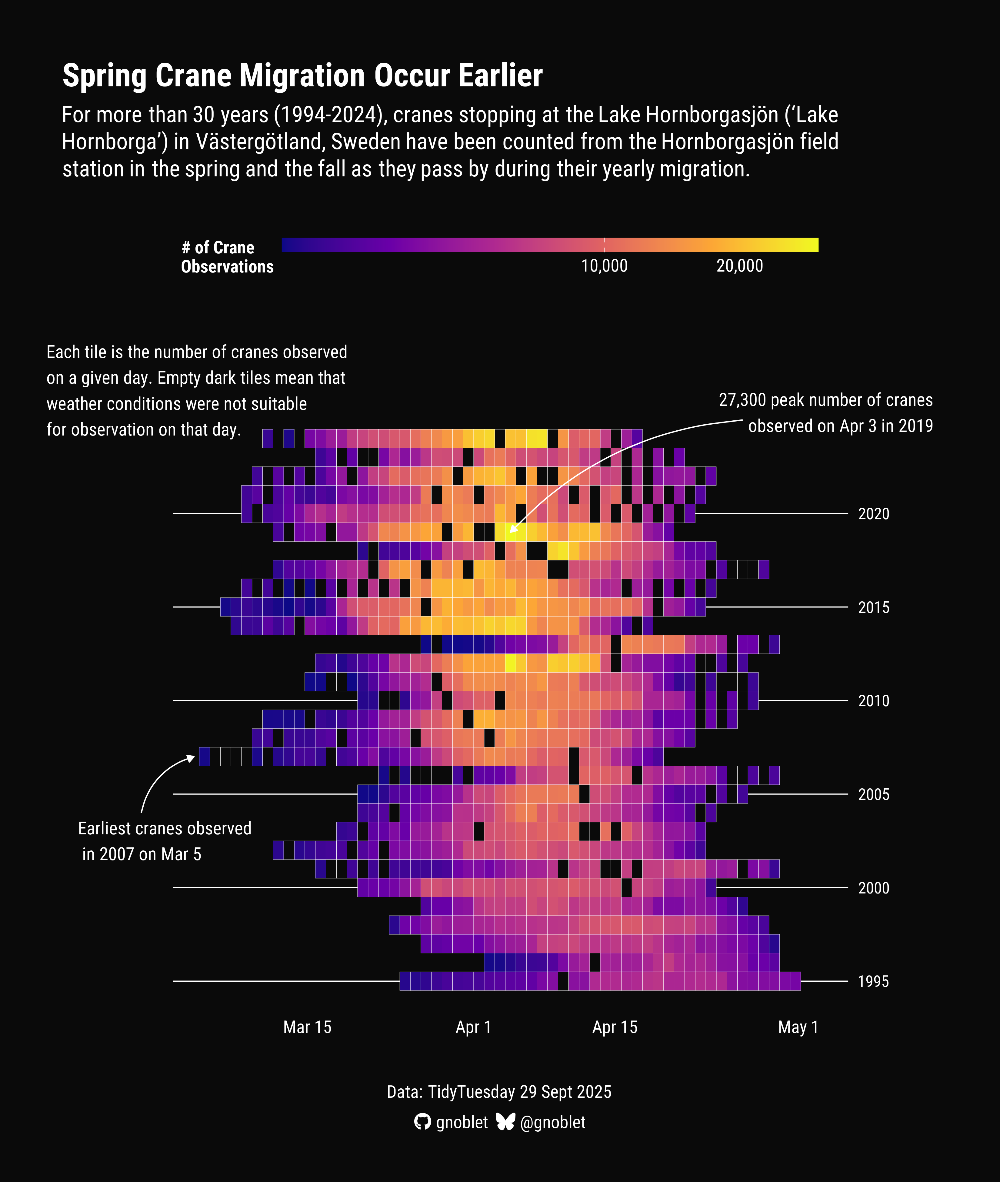
scale_fill_viridis_c(
name = "# of Crane\nObservations",
trans = "sqrt",
labels = scales::comma_format(),
option = "plasma",
na.value = "#0a0a0aff"
) +
scale_x_continuous(
limits = c(19, 105),
breaks = spring_breaks,
labels = spring_labels,
expand = c(0, 2)
) +
scale_y_continuous(
limits = c(1994, 2030),
breaks = c(1994, 2024),
expand = c(0, 1)
) +
labs(
title = title_text,
subtitle = subtitle_text,
x = NULL,
y = NULL
) +
# Add annotation for earliest 2007 data point
annotate(
"curve",
x = 28,
y = 2004,
xend = 33,
yend = 2007,
curvature = -0.3,
arrow = arrow(length = unit(0.01, "npc"), type = "closed"),
color = "white",
size = 0.5
) +
annotate(
"text",
x = 22,
y = 2002.5,
label = earliest_obs_text,
hjust = 0,
vjust = 0.5,
color = "white",
size = 5,
family = "Roboto Condensed"
) +
# Add annotation for max observation
annotate(
"curve",
x = 85,
y = 2025,
xend = max_obs_day,
yend = max_obs$year,
curvature = 0.2,
arrow = arrow(length = unit(0.01, "npc"), type = "closed"),
color = "white",
size = 0.5
) +
annotate(
"text",
x = 103,
y = 2025.4,
label = max_obs_text,
hjust = 1,
vjust = 0.5,
color = "white",
size = 5,
family = "Roboto Condensed"
) +
# Add annotation for explanation of tiles
annotate(
"text",
x = 19,
y = 2029,
label = exp_obs_text,
hjust = 0,
vjust = 1,
color = "white",
size = 5,
family = "Roboto Condensed"
) +
# Using ggplot2 4.0 theme features
theme_void(base_family = "Roboto Condensed") +
theme(
# Dark background theme using new ggplot2 4.0 approach
plot.background = element_rect(fill = "#0a0a0a", colour = NA),
panel.background = element_rect(fill = "#0a0a0a", colour = NA),
# Title styling with white text
plot.title = element_textbox_simple(
size = 26,
face = "bold",
colour = "white",
hjust = 0,
margin = margin(t = 20, b = 10, l = 30, r = 30)
),
plot.subtitle = element_textbox_simple(
size = 18,
colour = "white",
hjust = 0,
margin = margin(b = 30, l = 30, r = 30),
width = unit(0.9, "npc")
),
axis.text.x = element_text(
colour = "white",
size = 14,
hjust = 1
),
# Legend styling
legend.text = element_text(colour = "white", size = 14),
legend.title = element_text(colour = "white", size = 14, face = "bold", ),
legend.position = "top",
legend.key.height = unit(0.4, "cm"),
legend.key.width = unit(3, "cm"),
legend.margin = margin(t = 15, b = 20),
# Using new margin system from ggplot2 4.0
plot.margin = margin(30, 20, 30, 20)
) +
# Add branded footer using ggbranding
add_branding(
github = "gnoblet",
bluesky = "@gnoblet",
icon_color = "white",
text_color = "white",
additional_text = "Data: TidyTuesday 29 Sept 2025",
additional_text_color = "white",
caption_margin = margin(t = 40, b = 10),
line_spacing = 2L,
icon_size = "14pt",
text_size = "14pt",
caption_halign = 0.5
)