# Get data
tuesdata <- tt_load('2024-09-24')
cty <- tuesdata$country_results_df
ind <- tuesdata$individual_results_df
time <- tuesdata$timeline_dfInternational Mathematical Olympiad (IMO)
TidyTuesday Week 39
r
ggplot2
olympics
education
gender
Overview
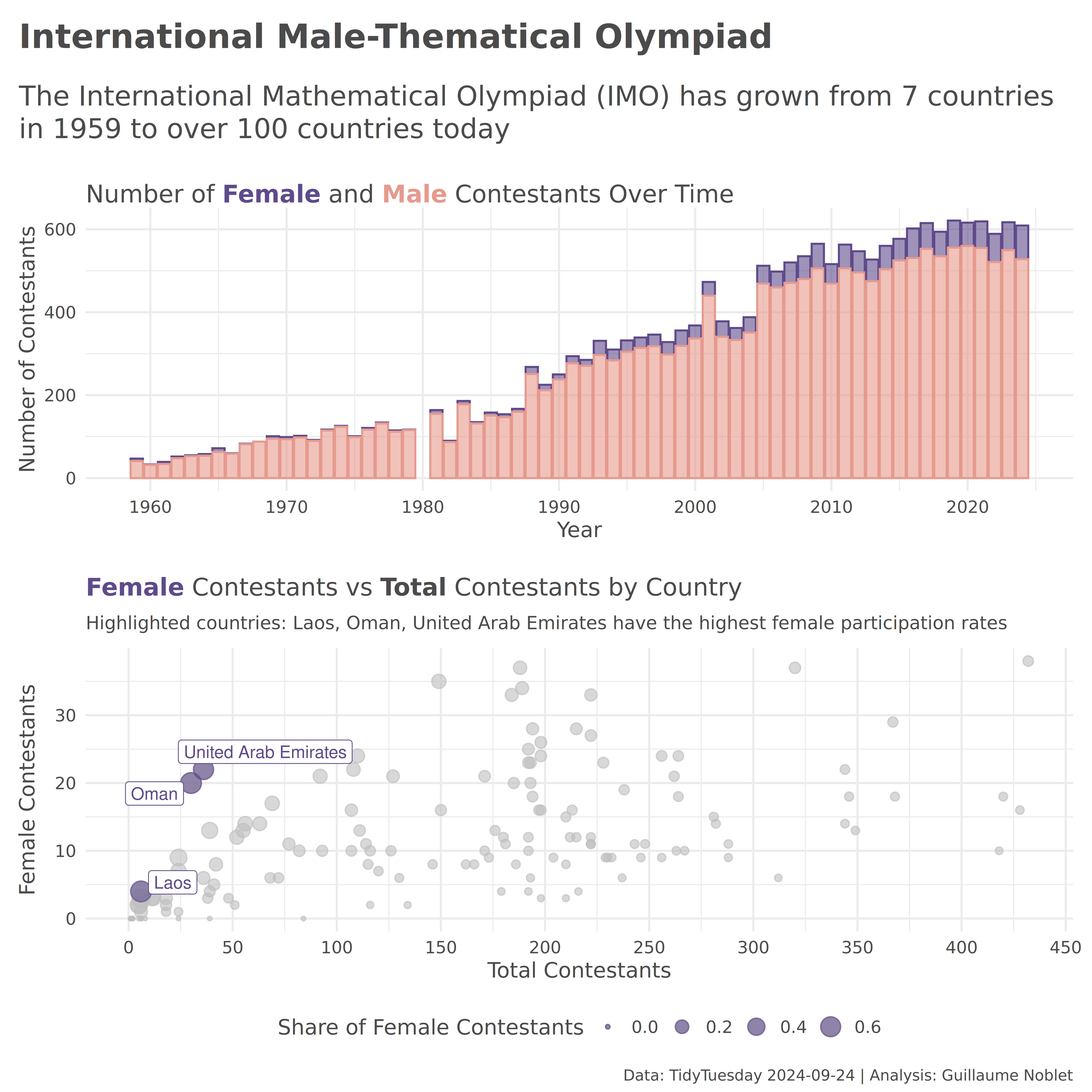
This week’s TidyTuesday explored the International Mathematical Olympiad (IMO) data, I look at gender participation patterns across countries and over time. The IMO is the World Championship Mathematics Competition for High School students, held annually since 1959.
Dataset
The IMO dataset includes: - Country-level results and team compositions - Individual contestant results - Timeline data showing participation trends - Gender breakdown of contestants by country and year
Analysis
Data Preparation
Gender Participation Over Time
# Prepare timeline data for gender analysis
time_longer <- time |>
  tyr$pivot_longer(
    cols = c(male_contestant, female_contestant, all_contestant),
    names_to = "gender",
    values_to = "n"
  ) |>
  dyr$mutate(gender = sgr$str_remove(gender, "_contestant")) |>
  dyr$select(year, country, countries, gender, n) |>
  dyr$group_by(year, gender) |>
  dyr$summarize(n = sum(n, na.rm = FALSE), .groups = "drop") |>
  dyr$filter(gender != "all")
Country-level Gender Analysis
# Analyze gender distribution by country
cty_gender_top_10 <- cty |>
  dyr$group_by(country) |>
  dyr$summarize(
    tot = sum(team_size_all, na.rm = TRUE),
    female = sum(team_size_female, na.rm = TRUE),
    .groups = "drop"
  ) |>
  dyr$mutate(share = female / tot)

# Get countries with highest female participation
cty_highest_share <- cty_gender_top_10 |>
  dyr$arrange(dyr$desc(share)) |>
  dyr$slice(1:3) |>
  dyr$pull(country)

# Get countries with no female contestants
cty_no_female <- cty_gender_top_10 |>
  dyr$filter(female == 0) |>
  nrow()

cat(
  "Countries with highest female participation:",
  paste(cty_highest_share, collapse = ", "),
  "\n"
)
Countries with highest female participation: Laos, Oman, United Arab Emirates cat("Countries with no female contestants:", cty_no_female, "\n")Countries with no female contestants: 11 Visualizations
Gender Participation Timeline
# Colors
female_col <- "#5F4B8BFF"
male_col <- "#E69A8DFF"

p1 <- gg$ggplot(time_longer) +
  gg$geom_col(
    gg$aes(x = year, y = n, color = gender, fill = gender),
    alpha = 0.6
  ) +
  gg$scale_color_manual(
    values = c(female_col, male_col),
    labels = c("Female", "Male")
  ) +
  gg$scale_fill_manual(
    values = c(female_col, male_col),
    labels = c("Female", "Male")
  ) +
  gg$labs(
    x = "Year",
    y = "Number of Contestants",
    color = "Gender",
    fill = "Gender",
    title = "Number of <b><span style='color:#5F4B8BFF'>Female</span></b> and <span style='color:#E69A8DFF'><b>Male</b></span> Contestants Over Time"
  ) +
  gg$scale_x_continuous(breaks = seq(1960, 2020, 10)) +
  gg$theme_minimal(base_size = 14, base_family = "roboto") +
  gg$theme(
    plot.title = ggt$element_textbox_simple(size = 16),
    legend.position = "none",
    text = gg$element_text(family = "roboto", colour = "#4c4b4c")
  )
Female Participation by Country
p2 <- gg$ggplot(cty_gender_top_10) +
  gg$geom_point(
    gg$aes(x = tot, y = female, size = share),
    color = female_col,
    alpha = 0.6
  ) +
  ggh$gghighlight(
    country %in% cty_highest_share,
    label_key = country,
    label_params = list(size = 4, color = female_col)
  ) +
  gg$labs(
    x = "Total Contestants",
    y = "Female Contestants",
    size = "Share of Female Contestants",
    title = "<b><span style='color:#5F4B8BFF'>Female</span></b> Contestants vs <b>Total</b> Contestants by Country",
    subtitle = paste(
      "Highlighted countries:",
      paste(cty_highest_share, collapse = ", "),
      "have the highest female participation rates"
    )
  ) +
  gg$scale_x_continuous(breaks = seq(0, 500, 50)) +
  gg$scale_y_continuous(breaks = seq(0, 100, 10)) +
  gg$theme_minimal(base_size = 14, base_family = "roboto") +
  gg$theme(
    plot.title = ggt$element_textbox_simple(
      size = 16,
      margin = gg$margin(t = 10, b = 10)
    ),
    plot.subtitle = ggt$element_textbox_simple(
      size = 12,
      margin = gg$margin(b = 10)
    ),
    legend.position = "bottom",
    text = gg$element_text(family = "roboto", colour = "#4c4b4c")
  )
Combined Analysis
# Create combined visualization
patchwork <- p1 /
  p2 +
  pw$plot_annotation(
    title = "<b>International Male-Thematical Olympiad</b>",
    subtitle = "The International Mathematical Olympiad (IMO) has grown from 7 countries in 1959 to over 100 countries today",
    caption = "Data: TidyTuesday 2024-09-24 | Analysis: Guillaume Noblet",
    theme = gg$theme(
      plot.title = ggt$element_textbox_simple(
        size = 22,
        margin = gg$margin(t = 10, b = 10)
      ),
      plot.subtitle = ggt$element_textbox_simple(
        size = 18,
        margin = gg$margin(t = 10, b = 20)
      ),
      plot.caption = gg$element_text(size = 10),
      text = gg$element_text(family = "roboto", colour = "#4c4b4c")
    )
  )
Save plot
gg$ggsave('week_39.png', plot = patchwork, height = 10, width = 10, dpi = 600)Technical Notes
- Used
gghighlightto emphasize countries with highest female participation - Combined timeline and scatter plot views using
patchwork - Color scheme designed to distinguish gender categories clearly
- Data includes participation from 1959 to recent years
Viz