# Libraries
library(giscoR)
library(sf)
library(terra)
library(elevatr)
library(dplyr)
library(tmap)
library(tmap.mapgl)
# Get Switzerland boundary
ch <- gisco_get_nuts(nuts_id = "CH") |>
st_transform(4326)
# Get elevation data for Switzerland
dem <- get_elev_raster(
ch,
z = 6,
clip = "locations"
)
# Convert to terra and mask
dem_terra <- rast(dem) |>
mask(vect(ch))
# Convert raster to polygons with elevation values
# This creates a polygon for each raster cell
ch_elev_poly <- as.polygons(dem_terra) |>
st_as_sf() |>
st_transform(4326)
# Rename the elevation column
names(ch_elev_poly)[1] <- "elevation"
# Remove any NA values
ch_elev_poly <- ch_elev_poly |>
filter(!is.na(elevation))
# Create 3D elevation map with tmap.mapgl
tmap_mode("maplibre")
tm_shape(ch_elev_poly) +
tm_polygons_3d(
fill = "elevation",
fill.scale = tm_scale_continuous(values = "turku"),
fill.legend = tm_legend(title = "Elevation (m)"),
height = "elevation"
) +
tm_view(
set_view = 2
) +
tm_basemap("carto.dark_matter")Day 05 - Earth (Classical Elements 1/4)
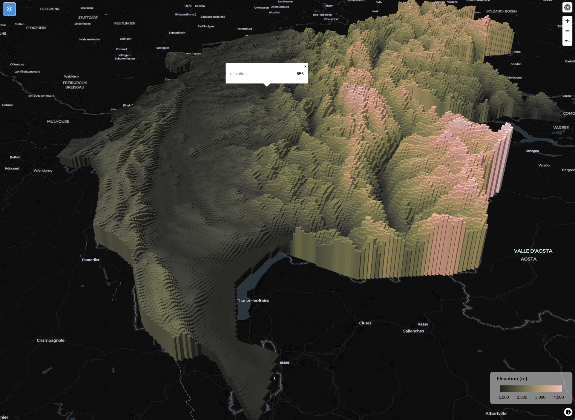
Let’s plot a 3D elevation map of Switzerland using R! We’ll use the giscoR package to get the country boundaries, the elevatr package to fetch elevation data, and the tmap and tmap.mapgl packages to create an interactive 3D map. Long time no see, tmap.