Day 03: Polygons

# Libraries
library(sf)
library(dplyr)
library(data.table)
library(janitor)
library(dplyr)
library(ggplot2)
library(patchwork)
library(viridis)
library(scico)
library(ggtext)
library(rnaturalearth)
library(rnaturalearthdata)

# Get admin2 polygons
admin2 <- st_read("agglo_communes/AGGLO_COMMUNES.shp", quiet = TRUE) |>
  st_transform(4326) |>
  mutate(
    COMMUNE = case_when(
      COMMUNE == "Genève (Ville)" ~ "Genève",
      COMMUNE == "Carouge" ~ "Carouge (GE)",
      COMMUNE == "Crans" ~ "Crans (VD)",
      COMMUNE == "Corsier (GE)" ~ "Corsier",
      COMMUNE == "Blonay" ~ "Blonay - Saint-Légier",
      COMMUNE == "Grand-Saconnex" ~ "Le Grand-Saconnex",
      COMMUNE == "Corsier" ~ "Corsier (GE)",
      .default = COMMUNE
    )
  )

# Load density per admin2 data and add sqrt transformation
dat <- fread("data.csv") |>
  clean_names() |>
  mutate(var = densite_dhabitants_2021, var_sqrt = var |> sqrt())

# Keep only admin2 in data
admin2 <- filter(
  admin2,
  COMMUNE %in% dat$libelle
)

# Merge data with spatial data
dat_sf <- merge(
  admin2,
  dat,
  by.x = "COMMUNE",
  by.y = "libelle",
  all.x = TRUE
)

# Extract percentiles and create classes
breaks <- quantile(dat_sf$var_sqrt, na.rm = TRUE, probs = seq(0, 1, 0.1))
dat_sf <- dat_sf |>
  mutate(
    cl = cut(var_sqrt, breaks = breaks, labels = LETTERS[1:10], include.lowest = TRUE)
  )


# Get swizerland lines
swiss_lines <- ne_states(country = "Switzerland", returnclass = "sf") 

# Find most and least dense cities (excluding NAs)
most_dense <- dat_sf |> 
  st_drop_geometry() |> 
  filter(!is.na(var)) |> 
  slice_max(var, n = 1)

least_dense <- dat_sf |> 
  st_drop_geometry() |> 
  filter(!is.na(var)) |> 
  slice_min(var, n = 1)

# Get centroids for annotations
most_dense_coords <- dat_sf |> 
  filter(COMMUNE == most_dense$COMMUNE) |> 
  st_centroid() |> 
  st_coordinates()

least_dense_coords <- dat_sf |> 
  filter(COMMUNE == least_dense$COMMUNE) |> 
  st_centroid() |> 
  st_coordinates()

# Colors - automatically map palette to classes
pal <- rev(scico(10, palette = 'acton')) |>
  setNames(LETTERS[1:10])

## Color for na values
na_col <- 'grey50'

# Color for admin2 borders
col_border <- '#437C90'

# Create custom theme
custom_theme <- theme_void(
  base_family = 'oswald'
)

# Fonts
showtext_auto()
showtext_opts(dpi = 600)
font_add_google("Oswald", "oswald")

# Main plot - map
p <- ggplot() +
  geom_sf(
    dat_sf,
    mapping = aes(fill = cl, color = cl),
  ) +
  # white lines for switzerland borders
  geom_sf(
    data = swiss_lines,
    fill = NA,
    color = "#ffffff",
    size = 1
  ) +
  # Annotation for most dense city
  annotate(
    "curve",
    x = most_dense_coords[1] - 0.28, 
    y = most_dense_coords[2] + 0.2,
    xend = most_dense_coords[1] - 0.02, 
    yend = most_dense_coords[2] + 0.02,
    arrow = arrow(length = unit(0.2, "cm"), type = "closed"),
    color = "#000000",
    curvature = 0.3,
    linewidth = 0.8
  ) +
  annotate(
    "text",
    x = most_dense_coords[1] - 0.45,
    y = most_dense_coords[2] + 0.24,
    label = paste0(most_dense$COMMUNE, " is the densest city\nwith ", round(most_dense$var), " hab/km²"),
    family = "oswald",
    size = 4.5,
    fontface = "bold",
    color = "#000000",
    hjust = 0
  ) +
  # Annotation for least dense city
  annotate(
    "curve",
    x = least_dense_coords[1] - 0.3,
    y = least_dense_coords[2] + 0.1,
    xend = least_dense_coords[1] - 0.05,
    yend = least_dense_coords[2] + 0.02,
    arrow = arrow(length = unit(0.2, "cm"), type = "closed"),
    color = "#260C3F",
    curvature = 0.3,
    linewidth = 0.6
  ) +
  annotate(
    "text",
    x = least_dense_coords[1] - 0.35,
    y = least_dense_coords[2] + 0.1,
    label = paste0(least_dense$COMMUNE, "\n(", round(least_dense$var), " hab/km²)"),
    family = "oswald",
    size = 5,
    fontface = "bold",
    color = "#260C3F",
    hjust = 1
  ) +
  coord_sf(
    xlim = c(5.75, 7.2),
    ylim = c(45.85, 46.62)
  ) +
  scale_fill_manual(values = pal, na.value = na_col) +
  scale_color_manual(values = pal, na.value = na_col) +
  guides(fill = 'none', color = "none") +
  custom_theme

# Set min value at 0 for color palette
breaks[1] = 0

tib <- tibble(
  end = breaks
) |> 
  mutate(
    start = lag(breaks, 1),
    cl = c(0, "A", "B", "C", "D", "E", 'F', 'G', 'H', 'I', 'J'),
    label = start ^ 2
  ) |> 
  # Remove first row
  slice(2:11)


# Legend plot
lg <- ggplot() +
  # Add color gradient
  geom_rect(
    data = tib,
    aes(xmin = start, xmax = end, ymin = 0, ymax = 1, fill = cl)
  ) +
  # Add labels
  geom_text(
    data = tib |> slice(c(seq(1, 10, 3))),
    mapping = aes(x = start, y = 1.1, label = round(label)),
    # angle = 45,
    hjust = 0.5,
    vjust = 0,
    color = "black"
  ) +
  # Add box behind points
  annotate(
    geom = "rect",
    xmin = 0,
    xmax = max(breaks),
    ymin = -1.25,
    ymax = -0.25,
    fill = NA,
    color = "black"
  ) +
  # Add jittered points
  geom_jitter(
    data = dat_sf |> st_drop_geometry(),
    mapping = aes(x = var_sqrt, y = -0.75, fill = cl, color = cl),
    pch = 21,
    # Control jitter amplitude
    width = 0,
    height = 0.5
  ) +
  # Scales 
  scale_y_continuous(limits = c(-1.5, 1.5)) +
  scale_fill_manual(values = pal, na.value = na_col) +
  scale_color_manual(values = pal, na.value = na_col) +
  guides(fill = 'none', color = 'none') +
  custom_theme

# Define layout
layout <- c(
  area(t = 0, l = 0, b = 10, r = 10),
  area(t = 11, l = 0, b = 14, r = 10)
)

# Combine plot and legend
final <- p + lg +
  plot_layout(design = layout) +
  plot_annotation(
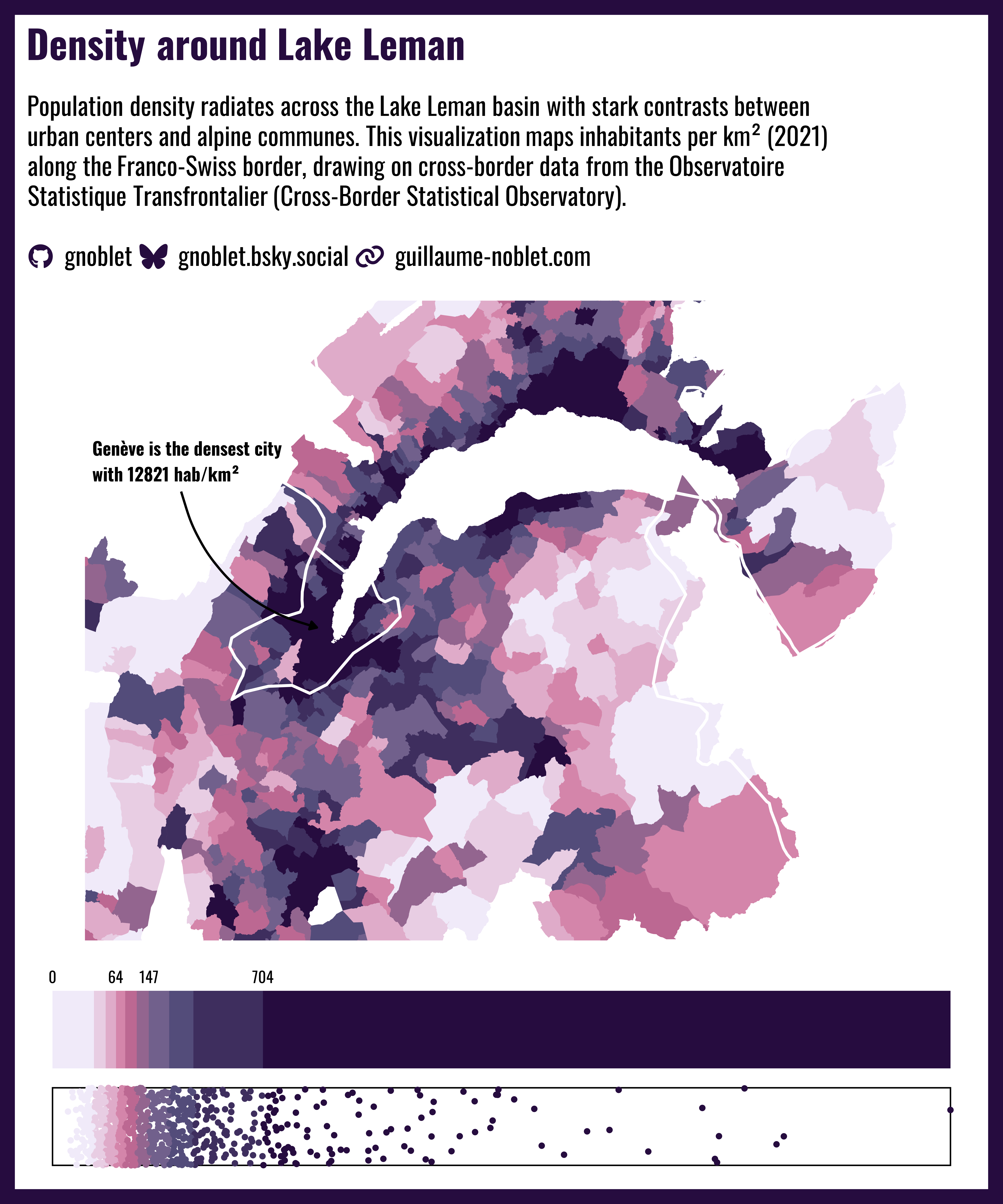
    title = 'Density around Lake Leman',
    subtitle = paste0("Population density radiates across the Lake Leman basin with stark contrasts between urban centers and alpine communes. This visualization maps inhabitants per km² (2021) along the Franco-Swiss border, drawing on cross-border data from the Observatoire Statistique Transfrontalier (<em>Cross-Border Statistical Observatory</em>).<br><br>",
    branding(
      github = "gnoblet",
      bluesky = "gnoblet.bsky.social",
      website = "guillaume-noblet.com",
      text_family = "oswald",
      text_color = "black",
      icon_color = "#260C3F",
      text_size = "18pt",
      icon_size = "18pt"
    ), "<br>"),
    theme = theme(
    plot.background = element_rect(fill = "#ffffffff", color = "#260C3F", linewidth = 10),
    text = element_text(family = 'oswald', hjust = 0.5, color = "#000000"),
    plot.title = element_textbox_simple(hjust = 0, face = 'bold', size = 28, margin = margin(t = 15, l = 15), width = unit(0.7, "npc"), color = "#260C3F"),
    plot.subtitle = element_textbox_simple(hjust = 0, size = 18, margin = margin(t = 20, l = 15), width = unit(0.85, "npc"))
  ) 
    ) 


# Save plot
ggsave("day_03.png", final, width = 10, height = 12, dpi = 600)